Rectangular coordinate system- a rectilinear coordinate system with mutually perpendicular axes on a plane or in space. The simplest and therefore most commonly used coordinate system. It is very easy and straightforward to generalize to spaces of any dimension, which also contributes to its wide application.
Related terms: Cartesian usually called a rectangular coordinate system with equal scales along the axes (so named after Rene Descartes), and general Cartesian coordinate system called an affine coordinate system (not rectangular).
Encyclopedic YouTube
-
1 / 5
A rectangular coordinate system on a plane is formed by two mutually perpendicular coordinate axes and O (\displaystyle O), which is called the origin of coordinates, the positive direction is chosen on each axis.
Point position A (\displaystyle A) on the plane is determined by two coordinates x (\displaystyle x) And y (\displaystyle y). Coordinate x (\displaystyle x) equal to the length of the segment O B, coordinate y (\displaystyle y)- length of the segment O C (\displaystyle OC) O B And O C (\displaystyle OC) are determined by lines drawn from the point A (\displaystyle A) parallel to the axes Y ′ Y (\displaystyle Y"Y) And X ′ X (\displaystyle X"X) respectively.
At this coordinate x (\displaystyle x) B (\displaystyle B) lies on the ray (and not on the ray O X (\displaystyle OX), as in the figure). Coordinate y (\displaystyle y) a minus sign is assigned if the point C (\displaystyle C) lies on the beam. Thus, O X ′ (\displaystyle OX") And O Y ′ (\displaystyle OY") are the negative directions of the coordinate axes (each coordinate axis is considered as a number axis).
Axis x (\displaystyle x) is called the abscissa axis, and the axis y (\displaystyle y)- ordinate axis. Coordinate x (\displaystyle x) called abscissa points A (\displaystyle A), coordinate y (\displaystyle y) - ordinate points A (\displaystyle A).
A (x , y) (\displaystyle A(x,\;y)) A = (x , y) (\displaystyle A=(x,\;y))or indicate that the coordinates belong to a specific point using an index:
x A , x B (\displaystyle x_(A),x_(B))Rectangular coordinate system in space(in this paragraph we mean three-dimensional space, about more multidimensional spaces - see below) is formed by three mutually perpendicular coordinate axes O X (\displaystyle OX), O Y (\displaystyle OY) And OZ (\displaystyle OZ). The coordinate axes intersect at the point O (\displaystyle O), which is called the origin of coordinates, on each axis a positive direction is selected, indicated by arrows, and a unit of measurement for the segments on the axes. The units of measurement are usually (not necessarily) the same for all axes. O X (\displaystyle OX)- x-axis, O Y (\displaystyle OY)- ordinate axis, OZ (\displaystyle OZ)- applicator axis.
Point position A (\displaystyle A) in space is determined by three coordinates x (\displaystyle x), y (\displaystyle y) And z (\displaystyle z). Coordinate x (\displaystyle x) equal to the length of the segment O B, coordinate y (\displaystyle y)- length of the segment O C (\displaystyle OC), coordinate z (\displaystyle z)- length of the segment O D (\displaystyle OD) in selected units of measurement. Segments O B, O C (\displaystyle OC) And O D (\displaystyle OD) are determined by planes drawn from the point A (\displaystyle A) parallel to the planes Y O Z (\displaystyle YOZ), X O Z (\displaystyle XOZ) And X O Y (\displaystyle XOY) respectively.
Coordinate x (\displaystyle x) called the abscissa of the point A (\displaystyle A), coordinate y (\displaystyle y)- ordinate of the point A (\displaystyle A), coordinate z (\displaystyle z)- applicate point A (\displaystyle A).
Symbolically it is written like this:
A (x , y , z) (\displaystyle A(x,\;y,\;z)) A = (x , y , z) (\displaystyle A=(x,\;y,\;z))or link a coordinate record to a specific point using an index:
x A , y A , z A (\displaystyle x_(A),\;y_(A),\;z_(A))Each axis is considered as a number line, i.e., it has a positive direction, and points lying on a negative ray are assigned negative coordinate values (the distance is taken with a minus sign). That is, if, for example, point B (\displaystyle B) lay not as in the picture - on the beam O X (\displaystyle OX), and on its continuation in reverse side from point O (\displaystyle O)(on the negative part of the axis O X (\displaystyle OX)), then the abscissa x (\displaystyle x) points A (\displaystyle A) would be negative (minus the distance O B). Likewise for the other two axes.
All rectangular coordinate systems in three-dimensional space are divided into two classes - rights(terms also used positive, standard) And left. Usually, by default, they try to use right-handed coordinate systems, and when depicting them graphically, they also place them, if possible, in one of several usual (traditional) positions. (Figure 2 shows a right-handed coordinate system.) It is impossible to combine the right and left coordinate systems by rotation so that the corresponding axes (and their directions) coincide. It is possible to determine which class any particular coordinate system belongs to using the right-hand rule, the screw rule, etc. (the positive direction of the axes is chosen so that when the axis is rotated O X (\displaystyle OX) counterclockwise by 90° its positive direction coincides with the positive direction of the axis O Y (\displaystyle OY), if this rotation is observed from the positive direction of the axis OZ (\displaystyle OZ)).
Rectangular coordinate system in multidimensional space
The rectangular coordinate system can be used in space of any finite dimension, in the same way as it is done for three-dimensional space. The number of coordinate axes is equal to the dimension of space (in this section we will denote it n).
To designate coordinates, they usually use not different letters, but the same letter with a numerical index. Most often this is:
x 1, x 2, x 3, … x n. (\displaystyle x_(1),x_(2),x_(3),\dots x_(n).)To denote arbitrary i The th coordinates from this set use a letter index:
and often the designation x i , (\displaystyle x_(i),) is also used to denote the entire set, implying that the index runs through the entire set of values: i = 1 , 2 , 3 , … n (\displaystyle i=1,2,3,\dots n).
In any dimension of space, rectangular coordinate systems are divided into two classes, right and left (or positive and negative). For multidimensional spaces, one of the coordinate systems is arbitrarily (conventionally) called right-handed, and the rest are right-handed or left-handed, depending on whether they are of the same orientation or not.
Rectangular vector coordinates
To define rectangular vector coordinates(applicable for representing vectors of any dimension) we can proceed from the fact that the coordinates of a vector (directed segment), the beginning of which is at the origin of coordinates, coincide with the coordinates of its end.
For vectors (directed segments) whose origin does not coincide with the origin of coordinates, rectangular coordinates can be determined in one of two ways:
- The vector can be moved so that its origin coincides with the origin of coordinates). Then its coordinates are determined in the manner described at the beginning of the paragraph: the coordinates of a vector translated so that its origin coincides with the origin of coordinates are the coordinates of its end.
- Instead, you can simply subtract the coordinates of its beginning from the coordinates of the end of the vector (directed segment).
- For rectangular coordinates, the concept of a vector coordinate coincides with the concept of an orthogonal projection of a vector onto the direction of the corresponding coordinate axis.
All operations on vectors are very simply written in rectangular coordinates:
- Addition and multiplication by scalar:
(This is true for any dimension n and even, on a par with rectangular ones, for oblique coordinates).
a ⋅ b = a 1 b 1 + a 2 b 2 + a 3 b 3 + ⋯ + a n b n (\displaystyle \mathbf (a) \cdot \mathbf (b) =a_(1)b_(1)+a_(2 )b_(2)+a_(3)b_(3)+\dots +a_(n)b_(n)) a ⋅ b = ∑ i = 1 n a i b i , (\displaystyle \mathbf (a) \cdot \mathbf (b) =\sum \limits _(i=1)^(n)a_(i)b_(i),)(Only in rectangular coordinates with unit scale on all axes).
- Using the scalar product you can calculate the length of the vector
- And k (\displaystyle \mathbf (k) )
e x (\displaystyle \mathbf (e)_(x)), e y (\displaystyle \mathbf (e)_(y)) And e z (\displaystyle \mathbf (e)_(z)).
Arrow symbols ( i → (\displaystyle (\vec (i))), j → (\displaystyle (\vec (j))) And k → (\displaystyle (\vec (k))) or e → x (\displaystyle (\vec (e))_(x)), e → y (\displaystyle (\vec (e))_(y)) And e → z (\displaystyle (\vec (e))_(z))) or others in accordance with the usual way of designating vectors in one or another literature.
In this case, in the case of a right coordinate system, the following formulas with vector products of unit vectors are valid:
For dimensions higher than 3 (or for the general case when the dimension can be any), usually for unit vectors we use notation with numerical indices instead, quite often this is
e 1 , e 2 , e 3 , … e n , (\displaystyle \mathbf (e) _(1),\mathbf (e) _(2),\mathbf (e) _(3),\dots \mathbf ( e) _(n),)Where n- dimension of space.
A vector of any dimension is expanded according to its basis (the coordinates serve as expansion coefficients):
a = a 1 e 1 + a 2 e 2 + a 3 e 3 + ⋯ + a n e n (\displaystyle \mathbf (a) =a_(1)\mathbf (e) _(1)+a_(2)\mathbf ( e) _(2)+a_(3)\mathbf (e) _(3)+\dots +a_(n)\mathbf (e) _(n)) a = ∑ i = 1 n a i e i , (\displaystyle \mathbf (a) =\sum \limits _(i=1)^(n)a_(i)\mathbf (e) _(i),) Pierre Fermat, however, his works were first published after his death. Descartes and Fermat used the coordinate method only on the plane.The coordinate method for three-dimensional space was first used by Leonhard Euler already in the 18th century. The use of orts apparently dates back to
1.10. RECTANGULAR COORDINATES ON MAPS
Rectangular coordinates (flat) - linear quantities: abscissa X and ordinateYdefining the position of points on a plane (on a map) relative to two mutually perpendicular axes X AndY(Fig. 14). Abscissa X and ordinateYpoints A- distances from the origin to the bases of the perpendiculars dropped from the point A on the corresponding axes, indicating the sign.
Rice. 14.Rectangular coordinates
In topography and geodesy, as well as on topographic maps, orientation is carried out in the north with angles counted clockwise, therefore, to preserve the signs of trigonometric functions, the position of the coordinate axes, accepted in mathematics, is rotated by 90°.
Rectangular coordinates on topographic maps of the USSR are applied by coordinate zones. Coordinate zones are parts of the earth's surface bounded by meridians with longitude divisible by 6°. The first zone is limited by meridians 0° and 6°, the second by b" and 12°, the third by 12° and 18°, etc.
The zones are counted from the Greenwich meridian from west to east. The territory of the USSR is located in 29 zones: from the 4th to the 32nd inclusive. The length of each zone from north to south is about 20,000 km. The width of the zone at the equator is about 670 km, at latitude 40° - 510 km, t latitude 50°-430 km, at latitude 60°-340 km.
All topographic maps within a given zone have a common rectangular coordinate system. The origin of coordinates in each zone is the point of intersection of the average (axial) meridian of the zone with the equator (Fig. 15), the average meridian of the zone corresponds to

Rice. 15.System of rectangular coordinates on topographic maps: a-one zone; b-parts of the zone
the abscissa axes, and the equator the ordinate axes. With this arrangement of coordinate axes, the abscissa of points located south of the equator and the ordinate of points located west of the middle meridian will have negative values. For the convenience of using coordinates on topographic maps, a conditional count of ordinates has been adopted, excluding negative ordinate values. This is achieved by the fact that the ordinates are counted not from zero, but from the value 500 km, That is, the origin of coordinates in each zone is, as it were, moved to 500 km left along the axisY.In addition, to unambiguously determine the position of a point in rectangular coordinates on globe to the coordinate valueYThe zone number (single or double digit number) is assigned to the left.
The relationship between conditional coordinates and their real values is expressed by the formulas:
X " = X-, Y = U-500,000,
Where X" And Y"-real ordinate values;X,Y-conditional values of ordinates. For example, if a point has coordinates
X = 5 650 450: Y= 3 620 840,
then this means that the point is located in the third zone at a distance of 120 km 840 m from the middle meridian of the zone (620840-500000) and north of the equator at a distance of 5650 km 450 m.
Full coordinates - rectangular coordinates, written (named) in full, without any abbreviations. In the example above, the full coordinates of the object are given:
X = 5 650 450; Y= 3620 840.
Abbreviated coordinates are used to speed up target designation on a topographic map; in this case, only tens and units of kilometers and meters are indicated. For example, the abbreviated coordinates of this object would be:
X = 50 450; Y = 20 840.
Abbreviated coordinates cannot be used for target designation at the junction of coordinate zones and if the area of operation covers a space of more than 100 km by latitude or longitude.
Coordinate (kilometer) grid - a grid of squares on topographic maps, formed by horizontal and vertical lines drawn parallel to the axes of rectangular coordinates at certain intervals (Table 5). These lines are called kilometer lines. The coordinate grid is intended for determining the coordinates of objects and plotting objects on a map according to their coordinates, for target designation, map orientation, measuring directional angles and for approximate determination of distances and areas.
Table 5 Coordinate grids on maps
Map scales
Dimensions of the sides of the squares
Areas of squares, sq. km
on the map, cm
on the ground, km
1:25 000
1
1:50 000
1:100 000
1:200 000
On a map at a scale of 1:500,000, the coordinate grid is not completely shown; only the outputs of kilometer lines are plotted on the sides of the frame (after 2 cm). If necessary, a coordinate grid can be drawn on the map along these outputs.
Kilometer lines on maps are marked at their boundary exits and at several intersections inside the sheet (Fig. 16). The outermost kilometer lines on the map sheet are signed in full, the rest are abbreviated with two numbers (i.e., only tens and units of kilometers are indicated). The labels on the horizontal lines correspond to the distances from the ordinate axis (equator) in kilometers. For example, signature 6082 in the right top corner shows that this line is located at a distance of 6082 from the equator km.
The labels of the vertical lines indicate the zone number (one or two first digits) and the distance in kilometers (always three digits) from the origin of coordinates, conventionally moved west of the middle meridian by 500 km. For example, the signature 4308 in the lower left corner means: 4 - zone number, 308 - distance from the conditional origin in kilometers.
An additional coordinate (kilometer) grid can be plotted on topographic maps at scales of 1:25,000, 1:50,000, 1:100,000 and 1:200,000 along the exits of kilometer lines in the adjacent western or eastern zone. Outputs of kilometer lines in the form of dashes with corresponding signatures are given on maps located 2° east and west of the boundary meridians of the zone.

rice. 16.Coordinate (kilometer) grid on a map sheet
An additional coordinate grid is intended to transform the coordinates of one zone into the coordinate system of another, neighboring zone.
In Fig. 17 lines on the outside of the western frame with signatures 81,6082 and on the northern side of the frame with signatures 3693, 94, 95, etc. indicate the outputs of kilometer lines in the coordinate system of the adjacent (third) zone. If necessary, an additional coordinate grid is drawn on a sheet of map by connecting lines of the same name on opposite sides of the frame. The newly constructed grid is a continuation of the kilometer grid of the map sheet of the adjacent zone and must completely coincide (close) with it when gluing the map.

Western (3rd) zone coordinate grid
Rice. 17. Additional coordinate grid
The operation of a CNC machine is closely related to coordinate systems.
The coordinate axes of the machine are usually parallel to the guides, which allows, when programming processing in the CP, to directly indicate the directions and magnitudes of movement of the working bodies.
In order to facilitate the operation of CNC machines, they have a single direction of coordinate axes, which is mandatory for all manufacturers.
As a unified coordinate system for all CNC machines in accordance with GOST 23597-79 (ST SEV 3135-81), a standard (right) Cartesian coordinate system is adopted, in which the X, Y, Z axes (Figure 4.5) indicate positive movements of the tools relative to moving parts of the machine.
The positive directions of movement of the workpiece relative to the stationary parts of the machine are indicated by the X`,Y`,Z` axes, directed opposite to the X,Y,Z axes. Thus, positive is always the direction of movement in which the tool and the workpiece move away from each other.
Fig.4.5. Standard coordinate system for CNC machine
Circular movements of the tool (for example, the angular displacement of the spindle axis of a milling machine) are denoted by the letters A (around the X axis), B (around the Y axis), C (around the Z axis), and circular movements of the workpiece (for example, program-controlled rotation of the table on the boring machine) - respectively, with the letters A, B, C. The concept of “circular movements” does not include rotation of the spindle carrying the tool or the spindle of the lathe.
To designate secondary angular movements around special axes, the letters D and E are used.
To indicate the direction of movement of two working bodies along one straight line, the so-called secondary axes are used: U (parallel to X), V (parallel to Y), W (parallel to Z). For three movements in one direction, the so-called tertiary axes are also used: P, Q, R (see Fig. 4.5).
For machines of different types and models, coordinate systems are placed differently, defining the positive directions of the axes and the position of the origin of coordinates.
The machine coordinate system, selected in accordance with the recommendations of GOST 23597-79 (Fig. 4.5), is usually called standard. In this system, the positive directions of the coordinate axes are determined by the right-hand rule. The thumb (Fig. 4.6) indicates the positive direction of the abscissa axis (X), the index finger - the ordinate axis (Y), the middle finger - the applicate axis (Z). The positive direction of rotations around these axes is determined by another right-hand rule. According to this rule, if you place your thumb in the direction of the axis, then the remaining bent fingers will indicate the positive direction of rotation.

Fig.4.6. Right hand rule for rectangular coordinate system
The orientation of the axes of the standard coordinate system on the machine is associated with the direction of movement when drilling on drilling, boring, milling and turning machines. The direction of removal of the drill from the workpiece is taken as positive for the Z axis, i.e. The Z axis is always connected to the rotating element of the machine - the spindle. The X axis is perpendicular to the Z axis and parallel to the workpiece mounting plane. If two axes correspond to this definition, then the X axis is taken to be the one along which the greatest movement of the machine unit is possible. With the X and Z axes known, the Y axis is uniquely determined from the condition of the axes being located in the right rectangular coordinate system.
4.1. RECTANGULAR COORDINATES
In topography, rectangular coordinates are most widely used. Let's take two mutually perpendicular lines on the plane - OX And OY. These lines are called coordinate axes, and their intersection point ( O) - the origin of coordinates.
Rice. 4.1. Rectangular coordinates
The position of any point on the plane can be easily determined by specifying the shortest distances from the coordinate axes to the given point. The shortest distances are perpendiculars. The perpendicular distances from the coordinate axes to a given point are called the rectangular coordinates of this point. Lines parallel to the axis X, are called coordinates XA , and parallel axes Y- coordinates atA .
The quarters of the rectangular coordinate system are numbered. They are counted clockwise from the positive direction of the abscissa axis - I, II, III, IV (Fig. 4.1).
The rectangular coordinates discussed are used on a plane. This is where they got their name flat rectangular coordinates. This coordinate system is used in small areas of terrain taken as a plane.4.2. ZONAL SYSTEM OF RECTANGULAR GAUSSian COORDINATES
When considering the issue of “Projection of topographic maps,” it was noted that the surface of the Earth is projected onto the surface of a cylinder, which touches the surface of the Earth along the axial meridian. In this case, not the entire surface of the Earth is projected onto the cylinder, but only a part of it, limited by 3° of longitude to the west and 3° to the east from the axial meridian. Since each of the Gaussian projections transfers onto the plane only a fragment of the Earth’s surface, limited by meridians through 6° of longitude, a total of 60 projections (60 zones) must be compiled onto the Earth’s surface. In each of the 60 projections, a separate rectangular coordinate system.
In each zone the axis X is the average (axial) meridian of the zone, located 500 km to the west from its actual position, and the axis Y- equator (Fig. 4.2).
Rice. 4.2. Rectangular coordinate system
on topographic mapsThe intersection of the extended axial meridian with the equator will be the origin of coordinates: x = 0, y = 0. The point of intersection of the equator and the actual central meridian has the coordinates : x = 0, y = 500 km.
Each zone has its own origin. The zones are counted from the Greenwich meridian to the east. The first six-degree zone is located between the Greenwich meridian and the meridian with eastern longitude 6º (axial meridian 3º). The second zone is 6º east. - 12º E (axial meridian 9º). Third zone - 12º east. - 18º east (axial meridian 15º). Fourth zone - 18º east. - 24º east (axial meridian 21º), etc.
The zone number is indicated in the coordinate at first digit. For example, record at = 4 525 340 means that the given point is in the fourth zone (first digit) at a distance 525 340 m from the axial meridian of the zone, located west of 500 km.To determine the zone number by geographic coordinates, you need to add 6 to the longitude expressed in integer degrees and divide the resulting amount by 6. As a result of the division, we leave only an integer.
Example. Determine the number of the Gaussian zone for a point having an eastern longitude of 18º10".
Solution. To the whole number of degrees of longitude 18 we add 6 and divide the sum by 6
(18 + 6) / 6 = 4.
Our map is in the fourth zone.Difficulties when using the zonal coordinate system arise in cases where topographic and geodetic work is carried out in border areas located in two adjacent (adjacent) zones. The coordinate lines of such zones are located at an angle to each other (Figure 4.3).
To eliminate emerging complications, a zone overlap strip , in which the coordinates of points can be calculated in two adjacent systems. The width of the overlap strip is 4°, 2° in each zone.
An additional grid on the map is applied only in the form of outputs of its lines between the minute and outer frames. Its digitization is a continuation of the digitization of the grid lines of the adjacent zone. Additional grid lines are signed outside the outer frame of the sheet. Consequently, on a map sheet located in the eastern zone, when connecting the same-name outputs of the additional grid, a kilometer grid of the western zone is obtained. Using this grid, you can determine, for example, the rectangular coordinates of a point IN in the rectangular coordinate system of the western zone, i.e. rectangular coordinates of points A And IN will be obtained in one coordinate system of the western zone.

Rice. 4.3. Additional kilometer lines at the borders of zones
On a 1:10,000 scale map, the additional grid is divided only on those sheets in which the eastern or western meridian of the inner frame (trapezoid frame) is the boundary of the zone. On topographical plans no additional mesh is applied.
4.3. DETERMINING RECTANGULAR COORDINATES USING A COMPASS METER
An important element topographic map(plan) is a rectangular grid. On all sheets of this 6-degree zone, the grid is applied in the form of rows of lines, parallel to the axial meridian and equator(Fig. 4.2). The vertical grid lines are parallel to the axial meridian of the zone, and the horizontal lines are parallel to the equator. Horizontal kilometer lines are counted from bottom to top, and vertical ones - from left to right. .
The intervals between lines on maps of scales 1:200,000 - 1:50,000 are 2 cm, 1:25,000 - 4 cm, 1:10,000 - 10 cm, which corresponds to an integer number of kilometers on the ground. Therefore, a rectangular mesh is also called kilometer, and its lines are kilometer.
The kilometer lines closest to the corners of the frame of the map sheet are signed with the full number of kilometers, the rest - with the last two digits. Inscription 60 65 (see Fig. 4.4) on one of the horizontal lines means that this line is 6065 km away from the equator (north): inscription 43 07 at the vertical line means that it is in the fourth zone and is 307 km east from the beginning of ordinate counting. If a three-digit number is written in small numbers near the vertical kilometer line, the first two indicate the zone number.Example. It is necessary to determine from the map the rectangular coordinates of a terrain point, for example, a point of the state geodetic network (GGS) with mark 214.3 (Fig. 4.4). First, write down (in kilometers) the abscissa of the south side of the square in which this point is located (i.e. 6065). Then, using a measuring compass and a linear scale, determine the length of the perpendicular Δх= 550 m, pubescent from given point to this line. The resulting value (in this case 550 m) is added to the abscissa of the line. The number 6,065,550 is the abscissa X GGS point.
The ordinate of the GGS point is equal to the ordinate of the western side of the same square (4307 km), added to the length of the perpendicular Δу= 250 m, measured on the map. The number 4,307,250 is the ordinate of the same point.
In the absence of a measuring compass, distances are measured with a ruler or strip of paper.
X = 6065550, at= 4307250
Rice. 4.4. Defining rectangular coordinates using a linear scale4.4. DETERMINING RECTANGULAR COORDINATES USING A COORDINATOMETER
Coordinator - a small square with two perpendicular sides. Along the internal edges of the rulers are scales, the lengths of which are equal to the length of the side of the coordinate cells of the map of a given scale. The divisions on the coordinate meter are transferred from the linear scale of the map.
The horizontal scale is aligned with the bottom line of the square (in which the point is located), and the vertical scale must pass through this point. The scales determine the distances from the point to the kilometer lines.
x A = 6135,350 y A = 5577,710
Rice. 4.5. Determining rectangular coordinates using a coordinate meter4.5. PLACING POINTS ON THE MAP AT SPECIFIED RECTANGULAR COORDINATES
To plot a point on a map according to given rectangular coordinates, proceed as follows: in the coordinate record, two-digit numbers are found that abbreviate the lines of the rectangular grid. Using the first number, a horizontal grid line is found on the map, and a vertical grid line is found using the second number. Their intersection forms the southwestern corner of the square in which the desired point lies. On the eastern and western sides of the square, two equal segments are laid from its southern side, corresponding on the map scale to the number of meters in the abscissa X . The ends of the segments are connected by a straight line and on it, from the western side of the square, a segment corresponding to the number of meters in the ordinate is plotted on the map scale; the end of this segment is the desired point.
4.6. CALCULATION OF FLAT RECTANGULAR GAUSSian COORDINATES BY GEOGRAPHICAL COORDINATES
Plane rectangular Gaussian coordinates X And at very difficult to relate to geographic coordinates φ (latitude) and λ (longitude) points earth's surface. Suppose that some point A has geographic coordinates φ And λ . Since the difference in the longitudes of the boundary meridians of the zone is 6°, then, accordingly, for each of the zones it is possible to obtain the longitudes of the extreme meridians: 1st zone (0° - 6°), 2nd zone (6° - 12°), 3rd zone (12° - 18°), etc. Thus, according to the geographical longitude of the point A you can determine the number of the zone in which this point is located. At the same time, longitude λ The axis of the axial meridian of the zone is determined by the formula
λ OS = (6°n - 3°),
wherein n- zone number.To define plane rectangular coordinates X And at by geographic coordinates φ And λ Let’s use the formulas derived for Krasovsky’s reference ellipsoid (the reference ellipsoid is a figure that is as close as possible to the figure of the Earth in the part on which a given state or group of states is located):
X = 6367558,4969 (φ glad ) − (a 0 − l 2 N)sinφ cosφ (4.1)
at(l) = lNcosφ (4.2)Formulas (4.1) and (4.2) use the following notation:
y(l) - distance from the point to the axial meridian of the zone;
l= (λ - λ OS ) - the difference between the longitudes of the determined point and the axial meridian of the zone);
φ glad - latitude of a point, expressed in radian measure;
N = 6399698,902 - cos 2φ;
A 0 = 32140,404 - cos 2 φ;
A 3 = (0,3333333 + 0,001123 cos 2 φ) cos 2φ - 0.1666667;
A 4 = (0,25 + 0,00252 cos 2φ) cos 2φ - 0.04166;
A 5 = 0,0083 - cos 2φ;
A 6 = (0.166 cos 2 φ - 0.084) cos 2 φ.
y" is the distance from the axial meridian located west of 500 km.According to formula (4.1), the coordinate value y(l) are obtained relative to the axial meridian of the zone, i.e. it can turn out with “plus” signs for the eastern part of the zone or “minus” signs for the western part of the zone. To record coordinates y in the zonal coordinate system, it is necessary to calculate the distance to a point from the axial meridian of the zone, located 500 km to the west (y"in the table ) , and write the zone number in front of the resulting value. For example, the value received is
y(l)= -303678.774 m in zone 47.
Then
at= 47 (500000.000 - 303678.774) = 47196321.226 m.
We use spreadsheets for calculations Microsoft XL .Example. Calculate the rectangular coordinates of a point having geographic coordinates:
φ = 47º02"15.0543"N; λ = 65º01"38.2456" east.To the table Microsoft XL enter the initial data and formulas (Table 4.1).
Table 4.1.
D
E
F
Parameter
Computations
hail
φ (deg)
D2+E2/60+F2/3600
φ (rad)
RADIANS(C3)
Cos 2φ
Zone No.
INTEGER((D8+6)/6)
λos (deg)
l (deg)
D11+E11/60+F11/3600
l (rad)
RADIANS(C12)
6399698,902-((21562,267-
(108.973-0.612*C6^2)*C6^2))*C6^2A 0
32140,404-((135,3302-
(0.7092-0.004*C6^2)*C6^2))*C6^2A 4
=(0.25+0.00252*C6^2)*C6^2-0.04166
A 6
=(0.166*C6^2-0.084)*C6^2
A 3
=(0.3333333+0.001123*C6^2)*C6^2-0.1666667
A 5
0.0083-((0.1667-(0.1968+0.004*C6^2)*C6^2))*C6^2
6367558.4969*C4-(((C15-(((0.5+(C16+C17*C20)*C20))
*C20*C14)))*C5*C6)
=((1+(C18+C19*C20)*C20))*C13*C14*C6
ROUND((500000+C23);3)
CONCATENATE(C9;C24)
View of the table after calculations (Table 4.2).
Table 4.2.
Parameter
Computations
hail
φ (deg, min, sec)
φ (degrees)
φ (radians)
Cos 2φ
λ (deg, min, sec)
Zone number
λos (deg)
l (min, sec)
l (degrees)
l (radians)
A 0
A 4
A 6
A 3
A 5
4.7. CALCULATION OF GEOGRAPHICAL COORDINATES USING FLAT RECTANGULAR GAUSSian COORDINATES
To solve this problem, recalculation formulas obtained for Krasovsky’s reference ellipsoid are also used.
Suppose we need to calculate geographic coordinates φ And λ points A by its flat rectangular coordinates X And at, specified in the zonal coordinate system. In this case, the coordinate value at written down indicating the zone number and taking into account the transfer of the axial meridian of the zone to the west by 500 km.
Pre-by value at find the number of the zone in which the point being determined is located, and use the zone number to determine the longitude λ o the axial meridian and by the distance from the point to the axial meridian referred to the west, find the distance y(l) from a point to the axial meridian of the zone (the latter can have a plus or minus sign).
Geographic coordinate values φ And λ on flat rectangular coordinates X And at found using the formulas:
φ = φ X - z 2 b 2 ρ″ (4.3)
λ = λ 0 + l (4.4)
l = zρ″ (4.5)In formulas (4.3) and (4.5):
φ x ″= β″ +(50221746 + cos 2 β)10-10sinβcosβ ρ″;
β″ = (X / 6367558.4969) ρ″; ρ″ = 206264.8062″ - number of seconds in one radian
z = У(L) / (Nx сos φx);
N x = 6399698.902 - cos 2 φ x;
b 2 = (0.5 + 0.003369 cos 2 φ x) sin φ x cos φ x;
b 3 = 0.333333 - (0.166667 - 0.001123 cos2 φ x) cos2 φ x;
b 4 = 0.25 + (0.16161 + 0.00562 cos 2 φ x) cos 2 φ x;
b 5 = 0.2 - (0.1667 - 0.0088 cos 2 φ x) cos 2 φ x.We use spreadsheets for calculations Microsoft XL .
Example. Calculate the geographic coordinates of a point using rectangular coordinates:
x = 5213504.619; y = 11654079.966.To the table Microsoft XL enter the initial data and formulas (Table 4.3).
Table 4.3.
1
Parameter
Calculation
Hail.
Min.
Sec.
2
1
X
5213504,619
2
at
11654079,966
4
3
No.*zones
IF(C3<1000000;
C3/100000;C3/1000000)5
4
Zone No.
INTEGER(C4)
6
5
λoos
C5*6-3
7
6
y"
C3-C5*1000000
8
7
y(l)
C7-500000
9
8
ρ″
206264,8062
10
9
β"
C2/6367558.4969*C9
11
10
β rad
RADIANS(C10/3600)
12
11
β
WHOLE
(C10/3600)WHOLE
((C10-D12*3600)/60)C10-D12*
3600-E12*6013
12
Sin β
SIN(C11)
14
13
Cos β
COS(C11)
15
14
Cos 2 β
C14^2
16
15
φ X "
C10+(((50221746+((293622+
(2350+22*C14^2)*C14^2))*C14^2)))
*10^-10*C13*C14*C917
16
φ X glad
RADIANS(C16/3600)
18
17
φ X
WHOLE
(C16/3600)WHOLE
((C16-D18*3600)/60)C16-D18*
3600-E18*6019
18
Sin φ.
SIN(C17)
20
19
Cosφ X
COS(C17)
21
20
Cos 2φ X
C20^2
22
21
N X
6399698,902-((21562,267-
(108.973-0.612*C21)*C21))*C2123
22
Ν X Cosφ X
C22*C20
24
23
z
C8/(C22*C20)
25
24
z 2
C24^2
26
25
b 4
0.25+(0.16161+0.00562*C21)*C21
27
26
b 2
=(0.5+0.003369*C21)*C19*C20
28
27
b 3
0.333333-(0.166667-0.001123*C21)*C21
29
28
b 5
0.2-(0.1667-0.0088*C21)*C21
30
29
C16-((1-(C26-0.12
*C25)*C25))*C25*C27*C931
30
φ
=INTEGER
(C30/3600)=INTEGER
((C30-D31*3600)/60)=C30-D31*
3600-E31*6032
31
l"
=((1-(C28-C29*C25)*C25))*C24*C9
33
32
l 0
=INTEGER
(C32/3600)=INTEGER
((C32-D33*3600)/60)=C32-D33*
3600-E33*6034
33
λ
C6+D33
View of the table after calculations (Table 4.4).
Table 4.4.
Parameter
Calculation
Hail.
Zone number*
Zone number
λoos (deg)
y"
β rad
Cos 2 β
φ X "
φ X glad
φ X
Cosφ X
Cos 2φ X
N X
Ν X Cosφ X
z 2
b 4
b 2
b 3
b 5
φ
l 0
λ
If the calculations are made correctly, copy both tables onto one sheet, hide the lines of intermediate calculations and the column No., and leave only the lines for entering the initial data and calculation results. We format the table and adjust the names of columns and columns at your discretion.
Worksheets might look like thisTable 4.5.

Notes.
1. Depending on the required accuracy, you can increase or decrease the bit depth.
2. The number of rows in the table can be reduced by combining calculations. For example, do not calculate the radians of an angle separately, but immediately write them in the formula =SIN(RADIANS(C3)).
3. Rounding in paragraph 23 of the table. 4.1. We produce for “clutch”. Number of digits in rounding 3.
4. If you do not change the format of the cells in the “Grad” and “Min” columns, then there will be no zeros before the numbers. The format change here is made only for visual perception (at the author's discretion) and does not affect the calculation results.
5. To avoid accidentally damaging formulas, you should protect the table: Service / Protect sheet. Before protecting, select the cells for entering the original data, and then: Cell format / Protection / Protected cell - uncheck the box.4.8. RELATIONSHIP OF FLAT RECTANGULAR AND POLAR COORDINATE SYSTEMS
The simplicity of the polar coordinate system and the possibility of constructing it relative to any point in the terrain taken as a pole led to its widespread use in topography. In order to connect together the polar systems of individual terrain points, it is necessary to move on to determining the position of the latter in a rectangular coordinate system, which can be extended to a much larger area. The connection between the two systems is established by solving direct and inverse geodetic problems.
Direct geodetic problem consists in determining the coordinates of the end point IN (Fig. 4.4) lines AB along its length G horizontal layoutd , directionα and coordinates of the starting point XA , atA .
Rice. 4.6. Solving direct and inverse geodetic problemsSo, if we accept the point A(Fig. 4.4) beyond the pole of the polar coordinate system, and the straight line AB- beyond the polar axis parallel to the axis OH, then the polar coordinates of the point IN will d And α . It is necessary to calculate the rectangular coordinates of this point in the system HOU.
From Fig. 3.4 it is clear that XIN differs from XA by the amount ( XIN - XA ) = Δ XAB , A atIN differs from atA by the amount ( atIN - atA ) = Δ atAB . Final coordinate differences IN and primary A line points AB Δ X and Δ at called coordinate increments . Coordinate increments are orthogonal projections of the line AB on the coordinate axis. Coordinates XIN And atIN can be calculated using the formulas:
XIN = XA + Δ XAB (4.1)
The increment values are determined from the right triangle DIA according to the given d and α, since the increments Δ X and Δ at are the legs of this right triangle:
atIN = atA + Δ atAB (4.2)Δ XAB =dcos α (4.3)
Δ atAB = dsin α (4.4)The sign of the coordinate increments depends on the position angle.
Table 4.1.
Substituting the value of increments Δ XAB and Δ atAB into formulas (3.1 and 3.2), we obtain formulas for solving the direct geodetic problem:
XIN = XA + dcos α (4.5)
atIN = atA + dsin α (4.6)Inverse geodetic problem consists in determining the length of the horizontal spacedand the direction α of line AB according to the given coordinates of its starting point A (xA, yA) and final point B (xB, yB). The direction angle is calculated using the legs of a right triangle:
tan α =
 (4.7)
(4.7)Horizontal layout d, determined by the formula:
d =
 (4.8)
(4.8)To solve direct and inverse geodetic problems, you can use spreadsheets Microsoft Excel .
Example.
Calculate rectangular coordinates of a point B(xIN ,atIN ).
Point given A with coordinates: XA = 6068318,25; atA = 4313450.37. Horizontal layout (d) between point A and dot IN equals 5248.36 m. The angle between the north direction of the axis OH and direction to the point IN(position angle - α ) is equal to 30º.Entering source data and formulas into spreadsheets Microsoft Excel (Table 4.2).
Table 4.2.
Initial data
XA
atA
Computations
Δ XAB =d cos α
B4*COS(RADIANS(B5))
Δ atAB = d sin α
B4*SIN(RADIANS(B5))
XIN
atIN
View of the table after calculations (Table 4.3).Table 4.3.
Initial data
XA
atA
Computations
Δ XAB =d cos α
Δ atAB = d sin α
XIN
atIN
Example.
Points specified A And IN with coordinates:
XA = 6068318,25; atA = 4313450,37;
XIN = 6072863,46; atIN = 4313450,37.
Calculate horizontal distance d between point A and dot IN, and also the angle α between the north direction of the axis OH and direction to the point IN.
Entering source data and formulas into spreadsheets Microsoft Excel (Table 4.4).Table 4.4.
View of the table after calculations (Table 4.5).Initial data
XA
atA
XIN
atIN
Computations
ΔхAB
ΔуAB
SQRT(B7^2+B8^2)
Tangent
Arctangent
Degrees
DEGREES(B11)
Choice
IF(B12<0;B12+180;B12)
Position angle (deg)
IF(B8<0;B13+180;B13)
Table 4.5.
Initial data
XA
atA
XIN
atIN
Computations
ΔхAB
ΔуAB
Tangent
Arctangent
Degrees
Choice
Position angle (deg)
If your calculations match those in the tutorial, hide the intermediate calculations, format and protect the table.
Video
Rectangular coordinatesQuestions and tasks for self-control
- What quantities are called rectangular coordinates?
- On what surface are rectangular coordinates used?
- What is the essence of the zonal rectangular coordinate system?
- What is the number of the six-degree zone in which the city of Lugansk is located with coordinates: 48°35′ N. 39°20′ E
- Calculate the longitude of the axial meridian of the six-degree zone in which Lugansk is located.
- How are x and y coordinates calculated in the rectangular Gaussian coordinate system?
- Explain the procedure for determining rectangular coordinates on a topographic map using a measuring compass.
- Explain the procedure for determining rectangular coordinates on a topographic map using a coordinate meter.
- What is the essence of the direct geodetic problem?
- What is the essence of the inverse geodetic problem?
- What quantity is called the coordinate increment?
- Define sine, cosine, tangent and cotangent of an angle.
- How can we apply the Pythagorean theorem on the relationship between the sides of a right triangle in topography?
If you are at some zero point and are wondering how many units of distance you need to go straight ahead and then straight to the right to get to some other point, then you are already using a rectangular Cartesian coordinate system on the plane. And if the point is located above the plane on which you stand, and to your calculations you add an ascent to the point along the stairs strictly upward also by a certain number of distance units, then you are already using a rectangular Cartesian coordinate system in space.
An ordered system of two or three intersecting axes perpendicular to each other with a common origin (origin of coordinates) and a common unit of length is called rectangular Cartesian coordinate system .
The name of the French mathematician René Descartes (1596-1662) is associated primarily with a coordinate system in which a common unit of length is measured on all axes and the axes are straight. In addition to the rectangular one, there is general Cartesian coordinate system (affine coordinate system). It may also include axes that are not necessarily perpendicular. If the axes are perpendicular, then the coordinate system is rectangular.
Rectangular Cartesian coordinate system on a plane has two axes and rectangular Cartesian coordinate system in space - three axes. Each point on a plane or in space is defined by an ordered set of coordinates - numbers corresponding to the unit of length of the coordinate system.
Note that, as follows from the definition, there is a Cartesian coordinate system on a straight line, that is, in one dimension. The introduction of Cartesian coordinates on a line is one of the ways by which any point on a line is associated with a well-defined real number, that is, a coordinate.
The coordinate method, which arose in the works of Rene Descartes, marked a revolutionary restructuring of all mathematics. It became possible to interpret algebraic equations (or inequalities) in the form of geometric images (graphs) and, conversely, to look for solutions to geometric problems using analytical formulas and systems of equations. Yes, inequality z < 3 геометрически означает полупространство, лежащее ниже плоскости, параллельной координатной плоскости xOy and located above this plane by 3 units.
Using the Cartesian coordinate system, the membership of a point on a given curve corresponds to the fact that the numbers x And y satisfy some equation. Thus, the coordinates of a point on a circle with a center at a given point ( a; b) satisfy the equation (x - a)² + ( y - b)² = R² .
Rectangular Cartesian coordinate system on a plane
Two perpendicular axes on a plane with a common origin and the same scale unit form Cartesian rectangular coordinate system on the plane . One of these axes is called the axis Ox, or x-axis , the other - the axis Oy, or y-axis . These axes are also called coordinate axes. Let us denote by Mx And My respectively, the projection of an arbitrary point M on the axis Ox And Oy. How to get projections? Let's go through the point M Ox. This straight line intersects the axis Ox at the point Mx. Let's go through the point M straight line perpendicular to the axis Oy. This straight line intersects the axis Oy at the point My. This is shown in the picture below.
x And y points M we will call the values of the directed segments accordingly OMx And OMy. The values of these directed segments are calculated accordingly as x = x0 - 0 And y = y0 - 0 . Cartesian coordinates x And y points M abscissa And ordinate . The fact that the point M has coordinates x And y, is denoted as follows: M(x, y) .
Coordinate axes divide the plane into four quadrant , the numbering of which is shown in the figure below. It also shows the arrangement of signs for the coordinates of points depending on their location in a particular quadrant.
In addition to Cartesian rectangular coordinates on a plane, the polar coordinate system is also often considered. About the method of transition from one coordinate system to another - in the lesson polar coordinate system .

Rectangular Cartesian coordinate system in space
Cartesian coordinates in space are introduced in complete analogy with Cartesian coordinates in the plane.
Three mutually perpendicular axes in space (coordinate axes) with a common origin O and with the same scale unit they form Cartesian rectangular coordinate system in space .
One of these axes is called an axis Ox, or x-axis , the other - the axis Oy, or y-axis , the third - axis Oz, or axis applicate . Let Mx, My Mz- projections of an arbitrary point M space on the axis Ox , Oy And Oz respectively.
Let's go through the point M OxOx at the point Mx. Let's go through the point M plane perpendicular to the axis Oy. This plane intersects the axis Oy at the point My. Let's go through the point M plane perpendicular to the axis Oz. This plane intersects the axis Oz at the point Mz.
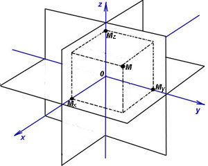
Cartesian rectangular coordinates x , y And z points M we will call the values of the directed segments accordingly OMx, OMy And OMz. The values of these directed segments are calculated accordingly as x = x0 - 0 , y = y0 - 0 And z = z0 - 0 .
Cartesian coordinates x , y And z points M are called accordingly abscissa , ordinate And applicate .
Coordinate axes taken in pairs are located in coordinate planes xOy , yOz And zOx .
Problems about points in a Cartesian coordinate system
Example 1.
A(2; -3) ;
B(3; -1) ;
C(-5; 1) .
Find the coordinates of the projections of these points onto the abscissa axis.
Solution. As follows from the theoretical part of this lesson, the projection of a point onto the abscissa axis is located on the abscissa axis itself, that is, the axis Ox, and therefore has an abscissa equal to the abscissa of the point itself, and an ordinate (coordinate on the axis Oy, which the x-axis intersects at point 0), which is equal to zero. So we get the following coordinates of these points on the x-axis:
Ax(2;0);
Bx(3;0);
Cx (-5; 0).
Example 2. In the Cartesian coordinate system, points are given on the plane
A(-3; 2) ;
B(-5; 1) ;
C(3; -2) .
Find the coordinates of the projections of these points onto the ordinate axis.
Solution. As follows from the theoretical part of this lesson, the projection of a point onto the ordinate axis is located on the ordinate axis itself, that is, the axis Oy, and therefore has an ordinate equal to the ordinate of the point itself, and an abscissa (coordinate on the axis Ox, which the ordinate axis intersects at point 0), which is equal to zero. So we get the following coordinates of these points on the ordinate axis:
Ay(0;2);
By(0;1);
Cy(0;-2).
Example 3. In the Cartesian coordinate system, points are given on the plane
A(2; 3) ;
B(-3; 2) ;
C(-1; -1) .
Ox .
Ox Ox Ox, will have the same abscissa as the given point, and an ordinate equal in absolute value to the ordinate of the given point, and opposite in sign. So we get the following coordinates of points symmetrical to these points relative to the axis Ox :
A"(2; -3) ;
B"(-3; -2) ;
C"(-1; 1) .
Example 4. Determine in which quadrants (quarters, drawing with quadrants - at the end of the paragraph “Rectangular Cartesian coordinate system on a plane”) a point can be located M(x; y) , If
1) xy > 0 ;
2) xy < 0 ;
3) x − y = 0 ;
4) x + y = 0 ;
5) x + y > 0 ;
6) x + y < 0 ;
7) x − y > 0 ;
8) x − y < 0 .
Example 5. In the Cartesian coordinate system, points are given on the plane
A(-2; 5) ;
B(3; -5) ;
C(a; b) .
Find the coordinates of points symmetrical to these points relative to the axis Oy .
Let's continue to solve problems together
Example 6. In the Cartesian coordinate system, points are given on the plane
A(-1; 2) ;
B(3; -1) ;
C(-2; -2) .
Find the coordinates of points symmetrical to these points relative to the axis Oy .
Solution. Rotate 180 degrees around the axis Oy directional segment from the axis Oy up to this point. In the figure, where the quadrants of the plane are indicated, we see that the point symmetrical to the given one relative to the axis Oy, will have the same ordinate as the given point, and an abscissa equal in absolute value to the abscissa of the given point and opposite in sign. So we get the following coordinates of points symmetrical to these points relative to the axis Oy :
A"(1; 2) ;
B"(-3; -1) ;
C"(2; -2) .
Example 7. In the Cartesian coordinate system, points are given on the plane
A(3; 3) ;
B(2; -4) ;
C(-2; 1) .
Find the coordinates of points symmetrical to these points relative to the origin.
Solution. We rotate the directed segment going from the origin to the given point by 180 degrees around the origin. In the figure, where the quadrants of the plane are indicated, we see that a point symmetrical to the given point relative to the origin of coordinates will have an abscissa and ordinate equal in absolute value to the abscissa and ordinate of the given point, but opposite in sign. So we get the following coordinates of points symmetrical to these points relative to the origin:
A"(-3; -3) ;
B"(-2; 4) ;
C(2; -1) .
Example 8.
A(4; 3; 5) ;
B(-3; 2; 1) ;
C(2; -3; 0) .
Find the coordinates of the projections of these points:
1) on a plane Oxy ;
2) on a plane Oxz ;
3) to the plane Oyz ;
4) on the abscissa axis;
5) on the ordinate axis;
6) on the applicate axis.
1) Projection of a point onto a plane Oxy is located on this plane itself, and therefore has an abscissa and ordinate equal to the abscissa and ordinate of a given point, and an applicate equal to zero. So we get the following coordinates of the projections of these points onto Oxy :
Axy (4; 3; 0);
Bxy (-3; 2; 0);
Cxy(2;-3;0).
2) Projection of a point onto a plane Oxz is located on this plane itself, and therefore has an abscissa and applicate equal to the abscissa and applicate of a given point, and an ordinate equal to zero. So we get the following coordinates of the projections of these points onto Oxz :
Axz (4; 0; 5);
Bxz (-3; 0; 1);
Cxz (2; 0; 0).
3) Projection of a point onto a plane Oyz is located on this plane itself, and therefore has an ordinate and applicate equal to the ordinate and applicate of a given point, and an abscissa equal to zero. So we get the following coordinates of the projections of these points onto Oyz :
Ayz(0; 3; 5);
Byz (0; 2; 1);
Cyz (0; -3; 0).
4) As follows from the theoretical part of this lesson, the projection of a point onto the abscissa axis is located on the abscissa axis itself, that is, the axis Ox, and therefore has an abscissa equal to the abscissa of the point itself, and the ordinate and applicate of the projection are equal to zero (since the ordinate and applicate axes intersect the abscissa at point 0). We obtain the following coordinates of the projections of these points onto the abscissa axis:
Ax(4;0;0);
Bx (-3; 0; 0);
Cx(2;0;0).
5) The projection of a point onto the ordinate axis is located on the ordinate axis itself, that is, the axis Oy, and therefore has an ordinate equal to the ordinate of the point itself, and the abscissa and applicate of the projection are equal to zero (since the abscissa and applicate axes intersect the ordinate axis at point 0). We obtain the following coordinates of the projections of these points onto the ordinate axis:
Ay(0; 3; 0);
By (0; 2; 0);
Cy(0;-3;0).
6) The projection of a point onto the applicate axis is located on the applicate axis itself, that is, the axis Oz, and therefore has an applicate equal to the applicate of the point itself, and the abscissa and ordinate of the projection are equal to zero (since the abscissa and ordinate axes intersect the applicate axis at point 0). We obtain the following coordinates of the projections of these points onto the applicate axis:
Az (0; 0; 5);
Bz (0; 0; 1);
Cz(0; 0; 0).
Example 9. In the Cartesian coordinate system, points are given in space
A(2; 3; 1) ;
B(5; -3; 2) ;
C(-3; 2; -1) .
Find the coordinates of points symmetrical to these points with respect to:
1) plane Oxy ;
2) planes Oxz ;
3) planes Oyz ;
4) abscissa axes;
5) ordinate axes;
6) applicate axes;
7) origin of coordinates.
1) “Move” the point on the other side of the axis Oxy Oxy, will have an abscissa and ordinate equal to the abscissa and ordinate of a given point, and an applicate equal in magnitude to the aplicate of a given point, but opposite in sign. So, we get the following coordinates of points symmetrical to the data relative to the plane Oxy :
A"(2; 3; -1) ;
B"(5; -3; -2) ;
C"(-3; 2; 1) .
2) “Move” the point on the other side of the axis Oxz to the same distance. From the figure displaying the coordinate space, we see that a point symmetrical to a given one relative to the axis Oxz, will have an abscissa and applicate equal to the abscissa and applicate of a given point, and an ordinate equal in magnitude to the ordinate of a given point, but opposite in sign. So, we get the following coordinates of points symmetrical to the data relative to the plane Oxz :
A"(2; -3; 1) ;
B"(5; 3; 2) ;
C"(-3; -2; -1) .
3) “Move” the point on the other side of the axis Oyz to the same distance. From the figure displaying the coordinate space, we see that a point symmetrical to a given one relative to the axis Oyz, will have an ordinate and an aplicate equal to the ordinate and an aplicate of a given point, and an abscissa equal in value to the abscissa of a given point, but opposite in sign. So, we get the following coordinates of points symmetrical to the data relative to the plane Oyz :
A"(-2; 3; 1) ;
B"(-5; -3; 2) ;
C"(3; 2; -1) .
By analogy with symmetrical points on a plane and points in space that are symmetrical to data relative to planes, we note that in the case of symmetry with respect to some axis of the Cartesian coordinate system in space, the coordinate on the axis with respect to which the symmetry is given will retain its sign, and the coordinates on the other two axes will be the same in absolute value as the coordinates of a given point, but opposite in sign.
4) The abscissa will retain its sign, but the ordinate and applicate will change signs. So, we obtain the following coordinates of points symmetrical to the data relative to the abscissa axis:
A"(2; -3; -1) ;
B"(5; 3; -2) ;
C"(-3; -2; 1) .
5) The ordinate will retain its sign, but the abscissa and applicate will change signs. So, we obtain the following coordinates of points symmetrical to the data relative to the ordinate axis:
A"(-2; 3; -1) ;
B"(-5; -3; -2) ;
C"(3; 2; 1) .
6) The applicate will retain its sign, but the abscissa and ordinate will change signs. So, we obtain the following coordinates of points symmetrical to the data relative to the applicate axis:
A"(-2; -3; 1) ;
B"(-5; 3; 2) ;
C"(3; -2; -1) .
7) By analogy with symmetry in the case of points on a plane, in the case of symmetry about the origin of coordinates, all coordinates of a point symmetrical to a given one will be equal in absolute value to the coordinates of a given point, but opposite to them in sign. So, we obtain the following coordinates of points symmetrical to the data relative to the origin.


